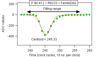
Figure A.1. An expanded view of the pulse shows the fitting range and the gaussian fit. The pulse shape is reasonably close to a gaussian, which is a preferred shape for Digital Pulse Processing.
We will now describe the analysis of the data file collected with the detector standing upright (the "vertical" geometry). We processed the ASCII event file with the help of IGOR 6.34. The framework for event processing is briefly explained on the offline analysis software page.
The basic analysis was aimed at the straightforward measurement of the cosmic mu-meson lifetime. The advanced analysis discussed later will enable us to improve the results of the basic approach.
We need to ask how to define the time of occurence of a pulse? In this particular experiment the position of the peak sample would provide sufficient timing precision (sample number 245 in the example above). However, we know from our previous studies that subnanosecond time resolution can be obtained by fitting the pulse with a gaussian function shown in red. Another method consists of calculating a weighted average over a range of samples encompassing the pulse. Stanley Paulauskas et al demonstrated that both methods could provide time resolution better than a nanosecond (NIM A737 (2014), page 22). We conclude that the time measurement will be affected more by the light collection within the scintillator rather than by the sampling clock period.
The gaussian fit and the weighted average are compared in Figure A.2. The left plot shows the entire experiment range. The right plot shows a small subrange to better assess the scatter. Both methods yield consistent results. We used the fitted centroid, but we could use the weighted average equally well.
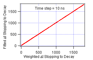
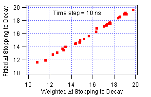
Figure A.3 shows the time differences between the first (leading) pulse and the second (trailing) pulse. The mu-meson decay is clearly visible up to ~6 microseconds, which is equal to about three mean lifetimes. (93% of all captured mu-mesons will decay within three lifetimes.) The time distribution becomes flat above this range, because no more mu-mesons are present. All the events in the flat portion of the plot are due to random coincidences. There were 45.8 such random coincidences per one microsecond in the flat portion of the distribution.
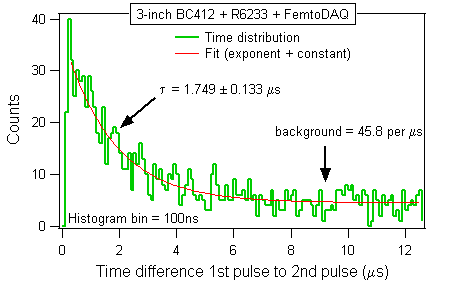
The exponent-plus-constant fit, shown with the red line in Figure A.3, yielded the mean lifetime of 1.75 microseconds, which is shorter than the official 2.2 microseconds. The discrepancy can be attributed to limited statistics of the true decays superimposed on the sizeable random background. The mean lifetime will be much better determined after removing the background.
We can now estimate the number of true mu-meson decays. We assume that the random coincidence density per microsecond is the same 45.8 in the entire coincidence window, also within the mu-meson decay range. Integrating this number over the full range we calculated that 554 out of 1,531 candidate events were due to mu-meson decay, while (1,531-554) = 997 events were due to random coincidences. The fraction of "true decays" among the recorded "decay candidates" was only 36%. (In other words, we recorded 64% random coincidences.)
One can ask why did we see so many random coincidences in this experiment? We point out that only one out of 6,339 passing mu-mesons was captured in the detector. (In total, FemtoDAQ processed 3,512,000 events, out of which only 554 were true mu-meson decays.) The probability that the mu-meson would stop in the detector was only 1.6e-4, what explains why it was so likely that two unrelated mu-mesons would conspire to produce two random pulses within the 20 microsecond coincidence window.
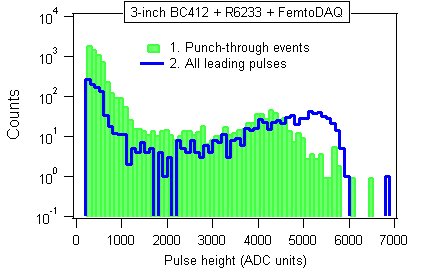
In this section we will use extra information which was present in the recorded waveforms. We will compare the pulse height (PH) distributions of three kinds of pulses:
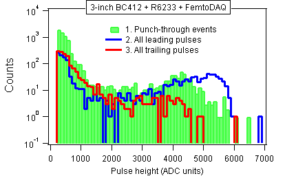
In all three cases we can see two components mixed in different proportions. The low energy component extends from zero up to PH=2000, while the high-energy "bump" is present for PH > 2000.
In the ideal case without random coincidences, the three kinds of pulses would be due to the mu-mesons that punched through the detector without stopping (1), the stopped mu-mesons (2), and the electrons emitted from the mu-meson decays (3). In our non-ideal case random coincidences are mixed into all three groups 1, 2, 3, thus precluding definite conclusions. We will approach this problem in the next subsection.
Now we want to gain insight into the nature of the background. We start with the pulse height scatter plot of the leading and the trailing pulses. In principle, we do not expect any correlation because the mu-meson decay is independent of how the particle was stopped in the detector. We will now verify our expectation.
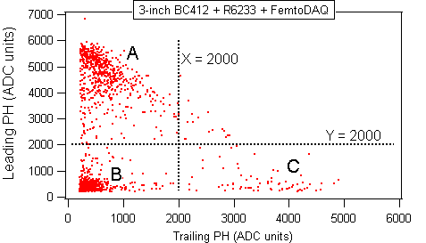
We can identify three groups of events A, B, C in Figure A.5. We can select any one of these groups using IF statements in the processing code. For example, IF (Leading_PH < 2000) will select both groups B and C together. Since C is low intensity compared to B, this statement effectively focuses the attention on B. Let us summarize:
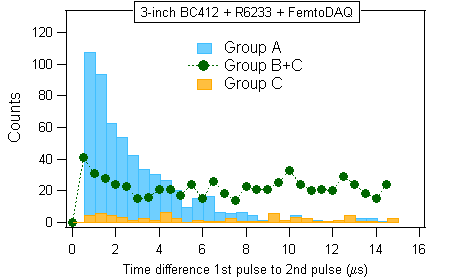
It now turns out that only group A corresponds to the mu-mesons that stopped and decayed in the detector. The other two groups B and C correspond to random background. There is some indication that group B also contains some "good events", but this may be due to the imperfect event selection. If we had more statistics then we could devise more stringent event selection criteria.
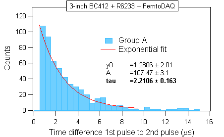
The cleaned distribution of the group A is repeated in the second panel together with the exponential fit. Focusing on A we extended the decay curve by one more mean lifetime of the mu-meson, up to ~8 microseconds. The mu-meson life time obtained from the clean distribution is in good agreement with the official value.
We have thus demonstrated that the random background can be suppressed using the event selection criteria derived from pulse amplitudes. We used a joint amplitude distribution (i.e., a scatter plot) to identify the suitable selections. At the end we used one-dimensional criteria (i.e., IF statements testing just a single quantity), but we had to see the scatter plot to understand the significance of the IF's. The 1D histograms in Figure A.4 did not provide sufficient insight to suspect that the IF statements could provide an effective method of background suppression.
Nuclear physics terminology: The IF statement would be called a gate in nuclear physics jargon. Since our IF's involved just a single quantity, they would be called one-dimensional gates. An IF involving more than a single quantity would be called a multi-dimensional gate. The gates are often implemented in "big science" using suitable NIM hardware such as Single Channel Analyzers (SCA) or Discriminator units. In digital electronics, the gates can be implemented inside the FPGA chips. In our example we first recorded the waveforms and then we implemented the gates in software in order to demonstrate the usefulness of this approach.
In the next step we will use the information gathered from Figure A.3 to clean the random background from the pulse height histograms shown in Figure A.4. We will subtract the random event contribution shown in green from the contaminated histogram shown in blue.
We estimated earlier that contaminated histograms were composed of 997 random events and 554 good events. The algorithm for background removal will work as follows:
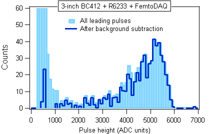
The result of the cleanup is shown in Figure A.8. We now see that the stopping mu-mesons deposit relatively large energies in the plastic medium. There is a low energy tail in the cleaned data, but the very low energy bump has now disappeared from the cleaned histogram. (The remaining "spike" at PH = 500 can be attributed to imperfect cleanup.) This observation agrees with our earlier finding that only the group A in Figure A.5 was due to stopping mu-mesons. Here we have arrived at the same conclusion using a different analysis method.
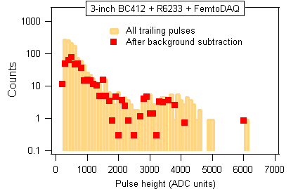
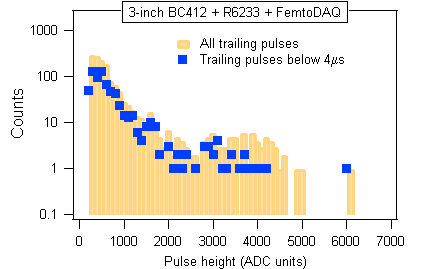
In the case of the trailing pulses (associated with the mu-meson decay) the result of the similar cleanup was less conclusive. We tried two different methods in Figure A.9.
The summary and conclusions are gathered on a separate page in order to avoid overloading this page with even more figures.